class: center, middle, inverse, title-slide # GGplot2 ## Visuals With GGplot2 ### Troy Funderburk ### 2019/13/05 (updated: 2019-05-20) --- class: inverse, center #Why Use GGplot2? ### Display Data - As each and every layer is added we must consider overall structure, local structure, and outliers. -- ### Create a Statistical Summary - model predictions surrounding the data. The data visualization helps improve our scientific model, the visual model provides subtle inferences that may be missed in ordinry literature. -- ### Metadata - This provides context tot he data itself through references and background nuance. This background data is meant to simply enahnce the data in the foreground, merely providing further context to the visualization. --- class: inverse, center # Different Options in GGplot2 ###Violin Plot ###Surface Plots ###Bar Graph ###Scatter Plots ###Box Plots --- class: center, inverse # The Violin Plot #####geom_violin() ```r library(ggplot2) ggplot(mpg, aes(drv, hwy)) + geom_violin() ``` <!-- --> --- class: center, inverse # How to make a 2D Image Look 3D With Surface Plots - ```r ggplot(faithfuld, aes(eruptions, waiting)) + geom_contour(aes(z = density, colour = ..level..)) ``` <!-- --> --- class: center, inverse # How to make a 2D Image Look 3D With Surface Plots cont.. ```r ggplot(faithfuld, aes(eruptions, waiting)) + geom_raster(aes(fill = density)) ``` <!-- --> --- class: center, inverse # Position Adjustments on Bar Graphs ###position_stack() stacks overlapping bars on top of eachother ###position_fill() stack bars so that the top is always number 1 ###position_dodge() place bars/boxes side by side --- class: center, inverse # Position Adjustments on Bar Graphs ```r dplot <- ggplot(diamonds, aes(color, fill = cut)) + xlab(NULL) + ylab(NULL) + theme(legend.position = "none") dplot + geom_bar() ``` <!-- --> --- class: center, inverse # Position Fill Example ```r dplot <- ggplot(diamonds, aes(color, fill = cut)) + xlab(NULL) + ylab(NULL) + theme(legend.position = "none") dplot + geom_bar(position = "fill") ``` 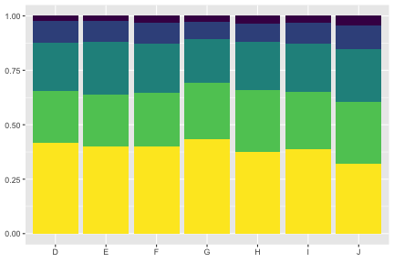<!-- --> --- class: center, inverse # Position Dodge Example ```r dplot <- ggplot(diamonds, aes(color, fill = cut)) + xlab(NULL) + ylab(NULL) + theme(legend.position = "none") dplot + geom_bar(position = "dodge") ``` 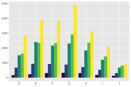<!-- --> --- class: center, inverse # Box Plot Examples ##### The box and whisker plots shows five summary statistics along with the individual outliers. Althought showing less than a histogram, it takes up far less space. ```r ggplot(diamonds, aes(carat, depth)) + geom_boxplot(aes(group = cut_width(carat, 0.1))) + xlim(NA, 2.05) ``` ``` ## Warning: Removed 997 rows containing missing values (stat_boxplot). ``` 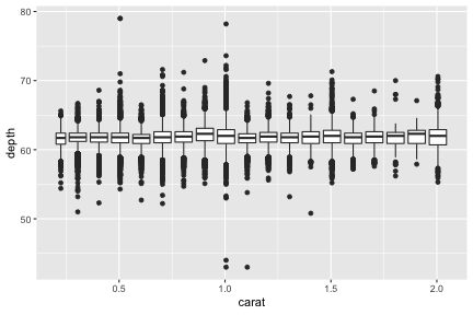<!-- --> --- class: center, inverse # Scatter Plot Examples ##### In this example we can see how ggplot auto picks colors based on the different factors. ```r ggplot(mpg, aes(displ, hwy, colour = factor(cyl))) + geom_point() ``` 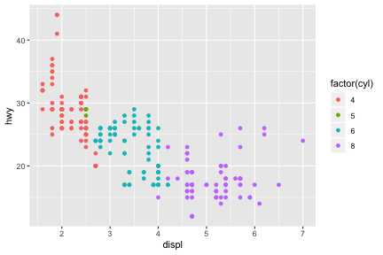<!-- --> --- class: center, inverse # When and Why To Set Limits -- ### Make limits smaller than data range to create emphasis -- ### Make range larger enabling plots to line up -- ```r df <- data.frame(x = 1:3, y = 1:3) base <- ggplot(df, aes(x, y)) + geom_point() print(base) ``` 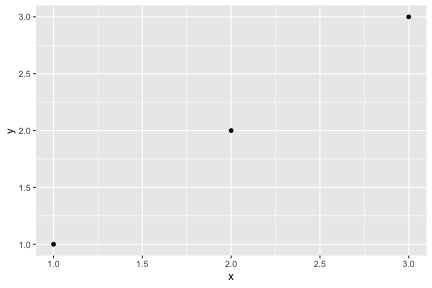<!-- --> --- class: center, inverse ```r base + scale_x_continuous(limits = c(0, 4)) ``` 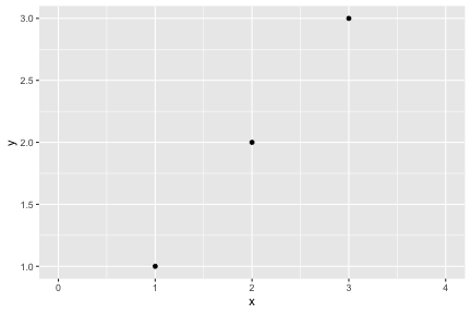<!-- --> --- class: center, inverse # Zooming Into a Plot -- ### coord_cartesian argues the xlim() and ylim() -- ```r base <- ggplot(mpg, aes(displ, hwy)) + geom_point() + geom_smooth() base ``` ``` ## `geom_smooth()` using method = 'loess' and formula 'y ~ x' ``` 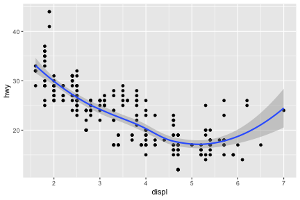<!-- --> --- class: center, inverse ```r base + scale_x_continuous(limits = c(5, 7)) ``` ``` ## `geom_smooth()` using method = 'loess' and formula 'y ~ x' ``` ``` ## Warning: Removed 196 rows containing non-finite values (stat_smooth). ``` ``` ## Warning: Removed 196 rows containing missing values (geom_point). ``` 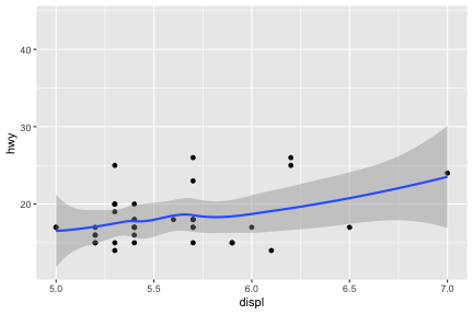<!-- --> --- class: center, inverse # Facet Wrapping ### Facettting is a mechanism for laying out multiple plots into subsets. These subsets are in individual panels. -- ```r mpg2 <- subset(mpg, cyl != 5 & drv %in% c("4", "f") & class != "2seater") base <- ggplot(mpg2, aes(displ, hwy)) + geom_blank() + xlab(NULL) + ylab(NULL) base + facet_wrap(~class, ncol = 3) ``` 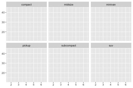<!-- --> ```r base + facet_wrap(~class, ncol = 3, as.table = FALSE) ``` 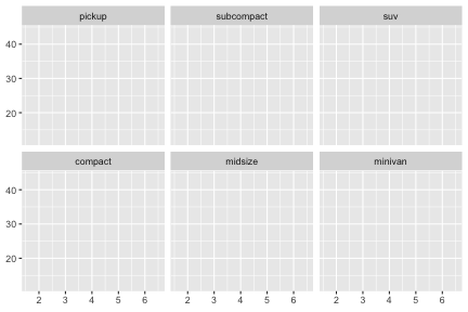<!-- --> --- class: center, inverse # Theme Elements ### 40 unique elements control appearance, grouped into 5 categories: plot, axis, legend, panel, and facet. --- class: center, inverse # Adjusting Themes in The Plot ```r base <- ggplot(mpg, aes(cty, hwy, color = factor(cyl)))+ geom_jitter() + geom_abline(colour = "grey50", size = 2) base ``` 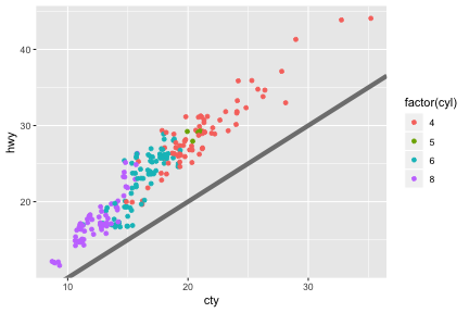<!-- --> --- class: center, inverse # Building on the simple version: ```r labelled <- base + labs(x = "city mileage/gallon",y = "highway mileage/gallon", colour = "cylinders", title = "Highway and city mileage are highly correlated") + scale_color_brewer(type = "seq", palette="Spectral") labelled ``` 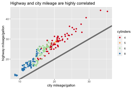<!-- --> --- class: center, inverse # A detailed version of the same plot: ```r styled <- labelled + theme_bw() + theme( plot.title = element_text(face = "bold", size = 12), legend.background = element_rect(fill = "white", size = 4, colour = "white"), legend.justification = c(0, 1),legend.position = c(0, 1), axis.ticks = element_line(colour = "grey70", size = 0.2), panel.grid.major = element_line(colour = "grey70", size = 0.2), panel.grid.minor = element_blank()) styled ``` 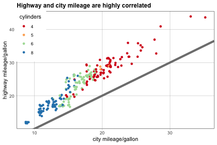<!-- --> --- class: center, inverse # Functional Programming ##### Rstudio treats all GGplot objects the same as regular r objects. You can add multiple geoms to the same base plot, giving you the user, a quick reference to multiple visuals. ```r geoms <- list( geom_point(), geom_boxplot(aes(group = cut_width(displ, 1))), list(geom_point(), geom_smooth())) p <- ggplot(mpg, aes(displ, hwy)) lapply(geoms, function(g) p + g) ``` ``` ## [[1]] ``` 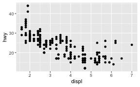<!-- --> ``` ## ## [[2]] ``` 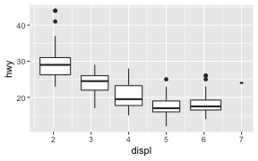<!-- --> ``` ## ## [[3]] ``` ``` ## `geom_smooth()` using method = 'loess' and formula 'y ~ x' ``` 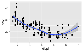<!-- --> --- class:inverse References Wickham, H. (2016) ggplot2. Elegant graphics for data analysis. Houston, Texas: Springer Nature. Wilkinson, L. (2005). The grammar of graphics. Statistics and computing, 2nd edn. Springer, New York